Ice edge detection & length estimation
Here, we go through a graphical approach to compute the length of the sea-ice edge. We will also take into account segments that represent closed contours around holes or sea-ice patches in the open ocean and exclude these from the total length.
First, let’s import the necessary libraries.
[1]:
import cmocean
import matplotlib.pyplot as plt
import cartopy.crs as ccrs
from tqdm.auto import tqdm
import numpy as np
import xarray as xr
from pyproj import Geod
from shapely.geometry import LineString, Point
from skimage import measure
Next, we will load sea-ice concentration data from the TOPAZ4 data set. The sea-ice edge is commonly defined as the 15% sea-ice concentration contour. For this example, we take only a single time step from the data set. We also constrain the domain slightly to focus only on the area of the Arctic where we have sea ice.
[2]:
file = "sic_topaz4.nc"
data = xr.open_dataset(file).siconc.squeeze().sel(x=slice(-25,15), y=slice(-25, 20));
data
/home/markusritschel/.local/lib/python3.10/site-packages/scipy/__init__.py:155: UserWarning: A NumPy version >=1.18.5 and <1.26.0 is required for this version of SciPy (detected version 1.26.4
  warnings.warn(f"A NumPy version >={np_minversion} and <{np_maxversion}"
[2]:
<xarray.DataArray 'siconc' (y: 361, x: 321)> Size: 464kB
[115881 values with dtype=float32]
Coordinates:
    time       datetime64[ns] 8B 2021-09-04
    longitude  (y, x) float32 464kB ...
    latitude   (y, x) float32 464kB ...
  * x          (x) float32 1kB -25.0 -24.88 -24.75 -24.62 ... 14.75 14.88 15.0
  * y          (y) float32 1kB -25.0 -24.88 -24.75 -24.62 ... 19.75 19.88 20.0
Attributes:
    standard_name:  sea_ice_area_fraction
    units:          1
    grid_mapping:   stereographic
cell_methods: area: meanUsing matplotlib
For a first try, we plot the 15% contour line via {func}matplotlib.pyplot.contour function.
[3]:
data.plot(cmap=cmocean.cm.ice)
CS = plt.contour(data.x, data.y, data, levels=[.15], colors='r')
contours = CS.allsegs[0]
The list contours containes the individual segments that {func}~matplotlib.pyplot.contour returns.
Next, we want to iterate over these segments, determine the length of each and check whether that feature is a closed ring or not.
Let’s look at one such segment:
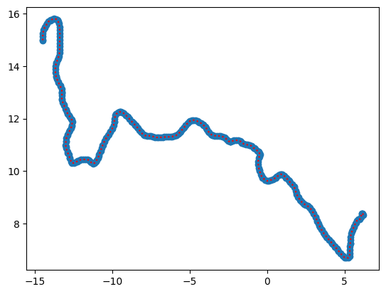
[4]:
seg = contours[25]
plt.scatter(*seg.T)
x,y = seg.T
plt.plot(x, y, ls=':', c='r');
Transform x/y coordinates from the plt.contour return to original lon/lat values
First, we build a trajectory of the segment x/y points
[10]:
ds_trajectory = xr.Dataset({
    'x': ('trajectory', seg.T[0]),
    'y': ('trajectory', seg.T[1])
})
ds_trajectory
[10]:
<xarray.Dataset> Size: 5kB
Dimensions:  (trajectory: 328)
Dimensions without coordinates: trajectory
Data variables:
    x        (trajectory) float64 3kB 6.211 6.182 6.125 ... -14.49 -14.5 -14.5
y (trajectory) float64 3kB 8.336 8.375 8.398 ... 15.12 15.0 14.97which we then use to select the points from the original dataset. Keep in mind that not neccessarily all points that are returned by the {func}~matplotlib.pyplot.contour function actually exist in the dataset. We therefore use the option method='nearest'.
[6]:
d = data.sel(x=ds_trajectory.x, y=ds_trajectory.y, method='nearest')
Let’s also adjust the longitudes to be in the desired range.
[7]:
adjusted_longitudes = np.where(d.longitude < 0, d.longitude + 360, d.longitude)
d['longitude'].values = adjusted_longitudes
# d = adjust_lons(d, 'longitude')
Now, we feed the longitude and latitude values to a {class}shapely.LineString object. {class}~shapely.LineString takes longitudes first, latitudes second.
[8]:
# import xoak
# data.xoak.set_index(['longitude', 'latitude'], xoak.index.scipy_adapters.ScipyKDTreeAdapter)

# lons = data.xoak.sel(longitude=ds_trajectory.longitude, latitude=ds_trajectory.latitude)
# lons
[9]:
lons = d.longitude.values
lats = d.latitude.values
ls = LineString(zip(lons, lats))
Plotting now the longitude and latitude values should give us the same result as the segment that {func}~matplotlib.pyplot.contour returned.
[11]:
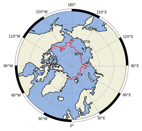
ax = plt.subplot(projection=ccrs.NorthPolarStereo())
data.plot(x='longitude', y='latitude', cmap=cmocean.cm.ice, ax=ax, transform=ccrs.PlateCarree())
ax.plot(lons, lats, transform=ccrs.PlateCarree(), c='r');
And we can also check the feature for being a closed feature (ring) and compute its length:
[12]:
geod = Geod(ellps="WGS84")
seg_len = geod.geometry_length(ls)/1e3

print(f"Is ring: {ls.is_ring}")
print(f"Segment length: {seg_len:.3f} km")
Is ring: False
Segment length: 3294.583 km
Great 💪 🚀
{admonition} Calculating the length :class: note There are different ways to determine the length of a trajectory on Earth. Here, we use {meth}`pyproj.Geod.geometry_length`. A comparison of different methods can be found [here](calculating-distances).
Apply it to the whole set of segments
Now, we can iterate over all segments and calculate the length of each segment and check it for being a ring (closed feature).
[13]:
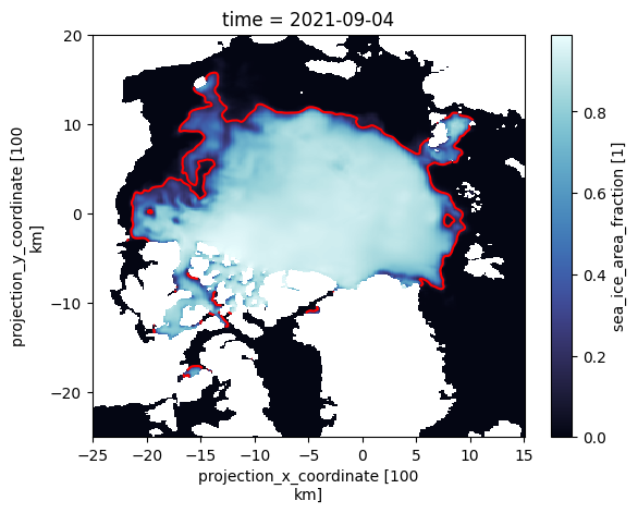
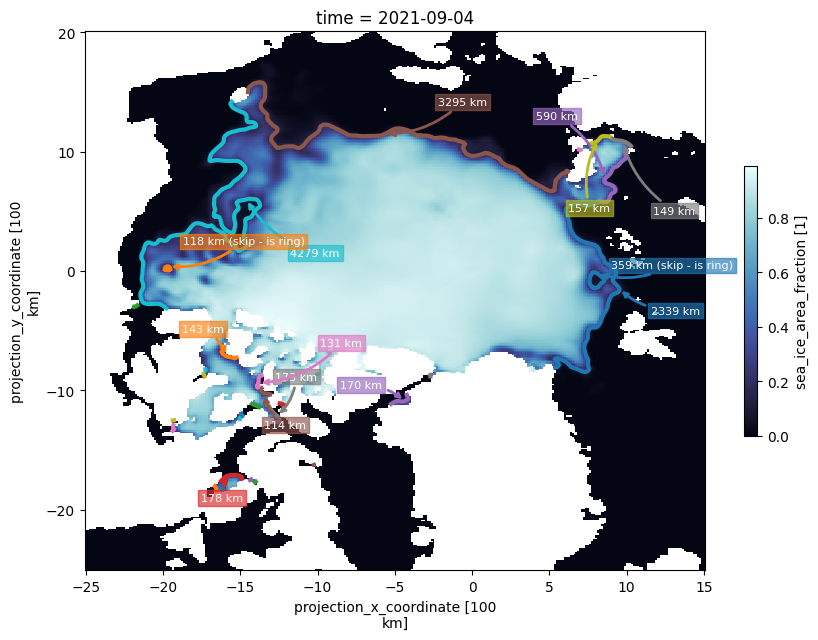
fig, ax = plt.subplots(figsize=(10,7))
data.plot(ax=ax, zorder=-10, cmap=cmocean.cm.ice, cbar_kwargs={'shrink': .5})

total_edge_length = []  # <-- Will contain the total length of the sea-ice edge, excluding the ring elements
for seg in tqdm(contours):
    # p = ax.plot(seg[:, 0], seg[:, 1], linewidth=3)
    p = ax.plot(*seg.T, linewidth=3)
    this_color = p[0].get_color()

    # lons = interpn((data.y, data.x), data.longitude.values, np.fliplr(seg))
    # lats = interpn((data.y, data.x), data.latitude.values, np.fliplr(seg))
    # lons = griddata(np.array(data.y, data.x), data.longitude.values, seg, method='cubic')
    # lats = griddata(np.array(data.y, data.x), data.latitude.values, seg, method='cubic')

    ds_trajectory = xr.Dataset({
        'x': ('trajectory', seg.T[0]),
        'y': ('trajectory', seg.T[1])
    })
    d = data.sel(x=ds_trajectory.x, y=ds_trajectory.y, method='nearest')
    adjusted_longitudes = np.where(d.longitude < 0, d.longitude + 360, d.longitude)
    d['longitude'].values = adjusted_longitudes
    # d = adjust_lons(d, 'longitude')

    lons = d.longitude.values
    lats = d.latitude.values
    ls = LineString(zip(lons, lats))

    geod = Geod(ellps="WGS84")
    seg_len = geod.geometry_length(ls)/1e3

    total_edge_length.append(seg_len)
    s = f"{seg_len:.0f} km"

    # Skip if polygon is shorter than 100 km
    if seg_len < 100:
        s += " (skip - too short)"
        print(s)
        continue
    # Also don't include segment in total length if polygon is ring and not around the pole
    elif ls.is_ring and not ls.contains(Point(0,0)):
        s += " (skip - is ring)"
        print(s)

    # Plot segments and annotations
    xy = seg[len(seg)//2,:]   # the middle coordinate value of the segment
    t = plt.annotate(s, xy, xytext=seg.mean(axis=0)+(np.random.randint(-6,6), np.random.randint(-6,6)),
                     arrowprops=dict(arrowstyle="->",
                                     edgecolor=this_color,
                                     lw=2,
                                     connectionstyle="arc3,rad=-0.2"),
                     fontsize='8', c='w')
    t.set_bbox(dict(facecolor=this_color, alpha=0.65, edgecolor=this_color, pad=2))

# plt.savefig("/home/u/u300917/sea-ice-edge-length.png", dpi=300)
print(f"Total length: {np.sum(total_edge_length):.3f} km")
53 km (skip - too short)
41 km (skip - too short)
12 km (skip - too short)
12 km (skip - too short)
0 km (skip - too short)
59 km (skip - too short)
12 km (skip - too short)
30 km (skip - too short)
25 km (skip - too short)
12 km (skip - too short)
59 km (skip - too short)
42 km (skip - too short)
12 km (skip - too short)
25 km (skip - too short)
0 km (skip - too short)
29 km (skip - too short)
0 km (skip - too short)
12 km (skip - too short)
359 km (skip - is ring)
118 km (skip - is ring)
Total length: 12631.450 km
Are the numbers reasonable?
For a comparison:
Greenland is approximately 2,670 kilometers (1,660 miles) long from its southernmost point to its northernmost point, as measured along the longitudinal line running through the center of the island.
Novaya Zemlya is approximately 650 kilometers (404 miles) long from its northernmost point to its southernmost point.
Using scikit-image
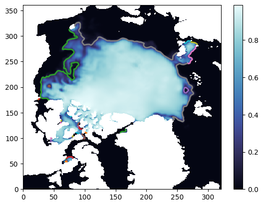
In a next approach, we use {func}skimage.measure.find_contours.
[14]:
contours = measure.find_contours(data.values, 0.15)

plt.pcolormesh(data, cmap=cmocean.cm.ice)
plt.colorbar()

for contour in contours:
    plt.plot(contour[:, 1], contour[:, 0], linewidth=2);
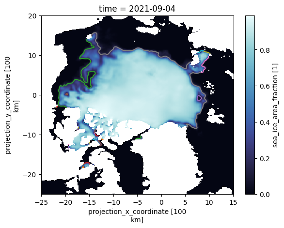
{admonition} Important Note that {func}`~skimage.measure.find_contours` returns the contours in axis coordinates, i.e. they origin at 0. Hence, we need to map them back to data coordinates.
[15]:
def mapme(x, y):
    x_ = ((data.x.max() - data.x.min()) / (data.x.size)).values * x
    y_ = ((data.y.max() - data.y.min()) / (data.y.size)).values * y
    x_ +=  data.x.min().values
    y_ +=  data.y.min().values
    return x_, y_
[16]:
data.plot(cmap=cmocean.cm.ice)

for contour in contours:
    seg_y, seg_x = contour.T
    seg_x, seg_y = mapme(seg_x, seg_y)
    plt.plot(seg_x, seg_y);
[17]:
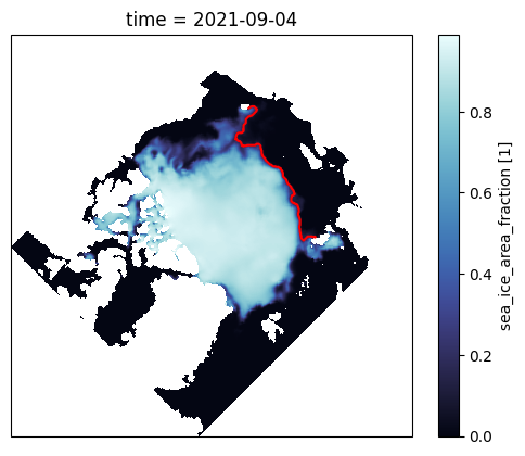
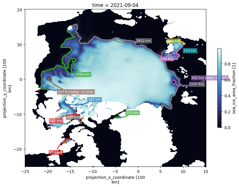
fig, ax = plt.subplots(figsize=(10,7))
data.plot(ax=ax, cmap=cmocean.cm.ice, cbar_kwargs={'shrink': .5})

total_edge_length = []  # <-- Will contain the total length of the sea-ice edge, excluding the ring elements
for seg in tqdm(contours):
    # p = ax.plot(seg[:, 0], seg[:, 1], linewidth=3)
    seg_x, seg_y = np.fliplr(seg).T
    seg_x, seg_y = mapme(seg_x, seg_y)
    seg = np.array([seg_x, seg_y]).T

    p = ax.plot(*seg.T, linewidth=3)
    this_color = p[0].get_color()

    # lons = interpn((data.y, data.x), data.longitude.values, np.fliplr(seg))
    # lats = interpn((data.y, data.x), data.latitude.values, np.fliplr(seg))
    # lons = griddata(np.array(data.y, data.x), data.longitude.values, seg, method='cubic')
    # lats = griddata(np.array(data.y, data.x), data.latitude.values, seg, method='cubic')

    ds_trajectory = xr.Dataset({
        'x': ('trajectory', seg.T[0]),
        'y': ('trajectory', seg.T[1])
    })
    d = data.sel(x=ds_trajectory.x, y=ds_trajectory.y, method='nearest')
    adjusted_longitudes = np.where(d.longitude < 0, d.longitude + 360, d.longitude)
    d['longitude'].values = adjusted_longitudes
    # d = adjust_lons(d, 'longitude')

    lons = d.longitude.values
    lats = d.latitude.values
    ls = LineString(zip(lons, lats))

    geod = Geod(ellps="WGS84")
    seg_len = geod.geometry_length(ls)/1e3

    total_edge_length.append(seg_len)
    s = f"{seg_len:.0f} km"

    # Skip if polygon is shorter than 100 km
    if seg_len < 100:
        s += " (skip - too short)"
        print(s)
        continue
    # Also don't include segment in total length if polygon is ring and not around the pole
    elif ls.is_ring and not ls.contains(Point(0,0)):
        s += " (skip - is ring)"
        print(s)

    # seg = seg.T

    # Plot segments and annotations
    xy = seg[len(seg)//2,:]   # the middle coordinate value of the segment
    t = plt.annotate(s, xy, xytext=seg.mean(axis=0)+(np.random.randint(-6,6), np.random.randint(-6,6)),
                     arrowprops=dict(arrowstyle="->",
                                     edgecolor=this_color,
                                     lw=2,
                                     connectionstyle="arc3,rad=-0.2"),
                     fontsize='8', c='w')
    t.set_bbox(dict(facecolor=this_color, alpha=0.65, edgecolor=this_color, pad=2))

# plt.savefig("/home/u/u300917/sea-ice-edge-length.png", dpi=300)
print(f"Total length: {np.sum(total_edge_length):.3f} km")
24 km (skip - too short)
60 km (skip - too short)
12 km (skip - too short)
46 km (skip - too short)
12 km (skip - too short)
17 km (skip - too short)
17 km (skip - too short)
59 km (skip - too short)
35 km (skip - too short)
30 km (skip - too short)
35 km (skip - too short)
79 km (skip - too short)
12 km (skip - too short)
12 km (skip - too short)
35 km (skip - too short)
12 km (skip - too short)
12 km (skip - too short)
402 km (skip - is ring)
133 km (skip - is ring)
Total length: 12843.677 km
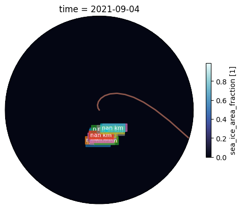
Finally, plot it on a map with correct stereographic projection
TBD
[18]:
from my_code_base.plot.maps import *

ax = plt.subplot(projection=ccrs.NorthPolarStereo())
# data = fix_overlap(data, ax, lon_name='longitude', lat_name='latitude')
# ax.polar.lat_limits = (65, 90)
# ax.polar.add_features()
data.plot(ax=ax, x='longitude', y='latitude', cmap=cmocean.cm.ice, cbar_kwargs={'shrink':.5}, transform=ccrs.PlateCarree())
# plt.pcolormesh(data.x, data.y, data, cmap=cmocean.cm.ice)
# plt.colorbar(shrink=.5)

total_edge_length = []
for seg in contours:
    # p = ax.plot(seg[:, 1], seg[:, 0], linewidth=3)
    # this_color = p[0].get_color()

    seg_x, seg_y = np.fliplr(seg).T
    seg_x, seg_y = mapme(seg_x, seg_y)
    seg = np.array([seg_x, seg_y])#.T

    # p = ax.plot(seg_x, seg_y, linewidth=3, transform=ccrs.PlateCarree())
    # this_color = p[0].get_color()

    ds_trajectory = xr.Dataset({
        'x': ('trajectory', seg_x),
        'y': ('trajectory', seg_y)
    })

    d = data.sel(x=ds_trajectory.x, y=ds_trajectory.y, method='nearest')
    adjusted_longitudes = np.where(d.longitude < 0, d.longitude + 360, d.longitude)
    d['longitude'].values = adjusted_longitudes

    # d = adjust_lons(d, 'longitude')
    lons = d.longitude.values
    lats = d.latitude.values
    ls = LineString(zip(lons, lats))

    p = ax.plot(lons, lats, linewidth=2, transform=ccrs.PlateCarree())
    this_color = p[0].get_color()

    # TODO: Check the difference between the following two variants!
    # Var 1
    geod = Geod(ellps="WGS84")
    seg_len = geod.geometry_length(ls)/1e3

    total_edge_length.append(seg_len)

    s = f"{seg_len:.0f} km"
    # Skip if polygon is ring and not around the pole
    if ls.is_ring and not ls.contains(Point(0,0)):
        s = "skip (is ring)"
        continue
    # also skip if polygon is shorter than 100 km
    elif seg_len < 100:
        s += " (skip)"
        print(s)
        continue

    # seg = np.fliplr(seg)
    seg = seg.T

    #plt.text(lons.mean(), lats.mean(), s)
    xy = seg[len(seg)//2,:]
    t = plt.annotate(s, xy, xytext=seg.mean(axis=0)+(np.random.randint(-6,6), np.random.randint(-6,6)),
                     arrowprops=dict(arrowstyle="->",
                                     edgecolor=this_color,
                                     lw=2,
                                     connectionstyle="arc3,rad=-0.2"),
                     fontsize='8', c='w', transform=ccrs.PlateCarree())
    t.set_bbox(dict(facecolor=this_color, alpha=0.65, edgecolor=this_color, pad=2))


# plt.savefig("/home/u/u300917/sea-ice-edge-length.png", dpi=300)
print(f"Total length: {np.sum(total_edge_length):.3f} km")
Total length: nan km
Plot ls
[40]:
from my_code_base.plot.maps import *

ax = plt.subplot(projection=ccrs.NorthPolarStereo())

# data_ = data.rename({'longitude':'lon', 'latitude':'lat'})
# data_ = fix_overlap(data_, ax)
# data_.plot.contour(x='lon', y='lat', ax=ax, levels=[.15], colors=['r'], zorder=10, alpha=.8)

for seg in tqdm(contours):
    ds_trajectory = xr.Dataset({
        'x': ('trajectory', seg.T[0]),
        'y': ('trajectory', seg.T[1])
    })

    d = data.sel(x=ds_trajectory.x, y=ds_trajectory.y, method='nearest')
    adjusted_longitudes = np.where(d.longitude < 0, d.longitude + 360, d.longitude)
    d['longitude'].values = adjusted_longitudes

    # d = adjust_lons(d, 'longitude')
    lons = d.longitude.values
    lats = d.latitude.values
    ls = LineString(zip(lons, lats))
    # ax.scatter(lons, lats, transform=ccrs.PlateCarree(), s=1)
    from cartopy.mpl.patch import geos_to_path
    from matplotlib.patches import PathPatch
    path, = geos_to_path(ls)
    patch = PathPatch(path, transform=ccrs.Geodetic(), edgecolor='r', facecolor='none')
    ax.add_patch(patch)
ax.polar.add_features()